Intro to Neural ODEs

ResNets

Neural ODEs comes from ResNets

As these models grew to hundreds of layers deep, ResNets’ performance decreased. Deep learning had reached its limit. We need state-of-the-art performance to train deeper networks.

在这里插入图片描述
It also directly adds the input to the output, this shortcut connection improves the model since, at the worst, the residual block does not do anything.

One final thought. A ResNet can be described by the following equation:

$$
h_{t+1} = h_{t}+f(h_{t},\theta_{t})
$$

h - value of the hidden layer;
t - tell us which layer we are look at

the next hidden layer is the sum of the input and a function of the input as we have seen.

Find introduction to ResNets in Reference

Euler’s Method

How Neural ODEs work

Above equation seems like calculus, and if you don’t remember from calculus class, the Euler’s method is the simplest way to approximate the solution of a differential equation with initial value.

$$
Initial value problem:y’(t)=f(t,y(t)), y(t_{0})=y_{0}
$$

$$
Euler’s Method: y_{n+1}=y_{n}+hf(t_{n},y_{n})
$$

through this we can find numerical approximation

Euler’s method and ResNets equation are identical, the only difference being the step size $h$, that is multiplied by the function. Because of this similarity, we can think ResNets is underlying differential equation.

Instead of going from diffeq to Euler’s method, we can reverse engineer the problem. Starting from the ResNet, the resulting differential equation is

$$
Neural ODE: {\frac{dh(t)}{dt}} = f(h(t),t,\theta)
$$

which describes the dynamics of our model.

The Basics

how a Neural ODE works

The Neural ODEs combines two concepts: deep learning and differential equations, we use the most simple methods - Euler’s method to make predictions.

Q:
How do we train it?
A:
Adjoint method

Include using another numerical solver to run backwards through time (backpropagating) and updating the model’s parameters.

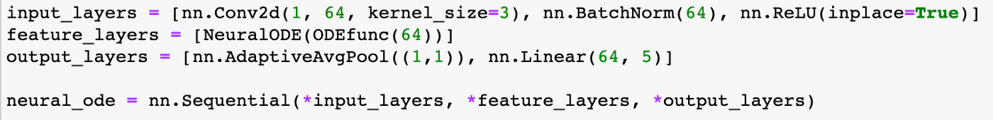
Defining the architecture:

在这里插入图片描述

Defining a neural ODE:

在这里插入图片描述

Put it all together into one:

在这里插入图片描述

Adjoint Method

part 3 - how a Neural ODE backpropagates with the adjoint method
this part - Adjoint Method

Model Comparison

Start with a simple machine learning model to showcase its strengths and weaknesses

ResNets model with lower time per epoch, and Neural ODEs model with more time.
ResNets model with more memory, and ODE model with O(1) space usage.

Overall, one of the main benefits is the constant memory usage while training the model. However, this comes at the cost of training time.

VAE[Variational Autoencoders]

Premise:

Generative model: Able to generate samples like those in training data

VAE is a directed generative model with observed and latent variables, which give us a atent space to sample from.

In view of the application that interpolate between sentences, Ｉ will use VAE to connect RNN and ODE．

VAE Architecture

在这里插入图片描述

VAE Design

When as Inference model, the input $x$ is passed to the encoder network, producing an approximate posterior $q(z|x)$ over latent variables.

Sentence prediction by conventional autoencoder

Sentences produced by greedily decoding from points between two sentence encodings with a conventional autoencoder. The intermediate sentences are not plausible English.

VAE Language Model

Words are represented using a learned dictionary of embedding words

VAE sentence interpolation

Paths between random points in VAE space

Intermediate sentences are grammatical

Topic and syntactic structure are consistent

Breakdown of another deep learning breakthrough

在这里插入图片描述

First, we encode the input sequence with some “standard” time series algorithms, let’s say RNN to obtain the primary embedding of the process
Run the embedding through the Neural ODE to get the “continuous” embedding
Recover initial sequence from the “continuous” embedding in VAE fashion

VAE as a generative model

variational autoencoder approach

A generative model through sampling procedure:

在这里插入图片描述
Training :

在这里插入图片描述

Define Model

class RNNEncoder(nn.moudle):
	def __init__(self,input_dim,hidden_dim,latent_dim):
		super(RNNEncoder,self).__init__()
		self.input_dim = input_dim
		self.hidden_dim = hidden_dim
		self.latent_dim = latent_dim

		self.rnn = nn.GRU(input_dim+1,hidden_dim)
		self.hid2lat = nn.Linear(hidden_dim,2*latent_dim)
	
	def forward(self,x,t):
		# Concatenate time to input
		t = t.clone()
		t[1:] = t[:-1] = t[1:]
		t[0] = 0
		xt = torch.cat((x,t),dim=-1)
		_,h0 = self.rnn(xt.flip((0,))) #Reversed
		# Compute latent dimension
		z0 = self.hid2lat(h0[0])
		z0_mean = z0[:,:self.latent_dim]
		z0_log_var = z0[:,self.latent_dim:]
		return z0_mean,z0_log_var

class NeuralODEDecoder(nn.Module):
	def __init__(self,output_dim,hidden_dim,latent_dim):
		super(NeuralODEDcoder,self).__init__()
		self.output_dim = output_dim
		self.hidden_dim = hidden_dim
		self.latent_dim = latent_dim
	
		func = NNODEF(latent_dim,hidden_dim,time_invariant=True)
		self.ode = NeuralODE(func)
		self.l2h = nn.Linear(latent_dim,hidden_dim)
		self.h2o = nn.Linear(hidden_dim,output_dim)

def forward(self,z0,t):
	zs = self.ode(z0,t,return_whole_sequence=True)
	hs = self.l2h(zs)
	xs = self.h2o(hs)
	return xs

class ODEVAE(nn.Module):
	def __init__(self,output_dim,hidden_dim,latent_dim):
		super(ODEVAE,self).__init__()
		self.output_dim = output_dim
		self.hidden_dim = hidden_dim
		self.latent_dim = latent_dim
		
		self.encoder = RNNEncoder(output_dim,hidden_dim,latent_dim)
		self.decoder = NeuralODEDecoder(output_dim,hidden_dim,latent_dim)

def forward(self,x,t,MAP=False):
	z_mean,z_log_var = self.encoder(x,t)
	if MAP:
		z = z_mean
	else:
		z = z_mean + torch.randn_like(z_mean)*torch.exp(0.5=z_log_var)
	x_p = self.decoder(z,t)
	return x_p,z,z_mean,z_log_var

def generate_with_seed(self,seed_x,t):
	seed_t_len = seed_x.shape[0]
	z_mean,z_log_var = self.encoder(seed_x,t[:seed_t_len])
	x_p = self.decoder(z_mean,t)
	return x_p