我们在收集到的数据中寻找合适的模型参数来使模型的预测价格与真实价格的误差最小。被训练的数据的集合称为训练数据集(training data set)或训练集(training set),每一条数据的主体作为一个样本(sample),被预测值称作标签(label),用来预测标签的因素叫作特征(feature)。特征用来表征样本的特点。
$$ l^{(i)}(\mathbf{w}, b) = \frac{1}{2} \left(\hat{y}^{(i)} - y^{(i)}\right)^2, $$
$$ L(\mathbf{w}, b) =\frac{1}{n}\sum_{i=1}^n l^{(i)}(\mathbf{w}, b) =\frac{1}{n} \sum_{i=1}^n \frac{1}{2}\left(\mathbf{w}^\top \mathbf{x}^{(i)} + b - y^{(i)}\right)^2. $$
# import packages and modules %matplotlib inline import torch from IPython import display from matplotlib import pyplot as plt import numpy as np import random
生成数据集
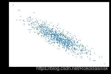
使用线性模型来生成数据集,生成一个 1000 个样本的数据集
1 2 3 4 5 6 7 8 9 10 11 12 13 14
# set input feature number num_inputs = 2 # set example number num_examples = 1000
# set true weight and bias in order to generate corresponded label true_w = [2, -3.4] true_b = 4.2
defdata_iter(batch_size, features, labels): num_examples = len(features) indices = list(range(num_examples)) random.shuffle(indices) # random read 10 samples for i in range(0, num_examples, batch_size): j = torch.LongTensor(indices[i: min(i + batch_size, num_examples)]) # the last time may be not enough for a whole batch yield features.index_select(0, j), labels.index_select(0, j)
batch_size = 10# read 10 samples for X, y in data_iter(batch_size, features, labels): # input features and labels print(X, '\n', y) break
初始化模型参数
1 2 3 4 5 6
# init parameter w = torch.tensor(np.random.normal(0, 0.01, (num_inputs, 1)), dtype=torch.float32) b = torch.zeros(1, dtype=torch.float32)
# define model deflinreg(X, w, b): return torch.mm(X, w) + b
定义损失函数
均方误差损失函数 $$ l^{(i)}(\mathbf{w}, b) = \frac{1}{2} \left(\hat{y}^{(i)} - y^{(i)}\right)^2, $$
1 2 3
# define loss function defsquared_loss(y_hat, y): return (y_hat - y.view(y_hat.size())) ** 2 / 2
定义优化函数
小批量随机梯度下降优化
1 2 3 4
# define optimization function defsgd(params, lr, batch_size): for param in params: param.data -= lr * param.grad / batch_size # ues .data to operate param without gradient track
# super parameters init lr = 0.03#学习率 num_epochs = 5#训练周期
net = linreg #单层网络 loss = squared_loss #均方误差损失函数
# training for epoch in range(num_epochs): # training repeats num_epochs times # in each epoch, all the samples in dataset will be used once # X is the feature and y is the label of a batch sample for X, y in data_iter(batch_size, features, labels): l = loss(net(X, w, b), y).sum() # calculate the gradient of batch sample loss l.backward() # using small batch random gradient descent to iter model parameters sgd([w, b], lr, batch_size) # reset parameter gradient w.grad.data.zero_()#参数梯度清零,为防止叠加 b.grad.data.zero_() train_l = loss(net(features, w, b), labels) print('epoch %d, loss %f' % (epoch + 1, train_l.mean().item()))
检验训练结果
1 2
# output result of trainning w, true_w, b, true_b
使用 torch 简化代码
未单独重写的步骤默认与上一致
读取数据集
1 2 3 4 5 6 7 8 9 10 11 12 13 14 15 16 17 18
import torch.utils.data as Data
batch_size = 10
# combine featues and labels of dataset dataset = Data.TensorDataset(features, labels)
# put dataset into DataLoader data_iter = Data.DataLoader( dataset=dataset, # torch TensorDataset format batch_size=batch_size, # mini batch size shuffle=True, # whether shuffle the data or not num_workers=2, # read data in multithreading )
for X, y in data_iter: print(X, '\n', y) break
定义模型
1 2 3 4 5 6 7 8 9 10 11
classLinearNet(nn.Module): def__init__(self, n_feature): super(LinearNet, self).__init__() # call father function to init self.linear = nn.Linear(n_feature, 1) # function prototype: `torch.nn.Linear(in_features, out_features, bias=True)`
defforward(self, x): y = self.linear(x) return y net = LinearNet(num_inputs) print(net) #单层线性网络
初始化模型参数
1 2 3 4 5 6 7
from torch.nn import init
init.normal_(net[0].weight, mean=0.0, std=0.01) init.constant_(net[0].bias, val=0.0) # or you can use `net[0].bias.data.fill_(0)` to modify it directly
for param in net.parameters(): print(param)
定义损失函数
1 2
loss = nn.MSELoss() # nn built-in squared loss function # function prototype: `torch.nn.MSELoss(size_average=None, reduce=None, reduction='mean')`
定义优化函数
1 2 3 4
import torch.optim as optim #随机梯度下降 optimizer = optim.SGD(net.parameters(), lr=0.03) # built-in random gradient descent function print(optimizer) # function prototype: `torch.optim.SGD(params, lr=, momentum=0, dampening=0, weight_decay=0, nesterov=False)`
训练
1
2
3
4
import torch.optim as optim #随机梯度下降 optimizer = optim.SGD(net.parameters(), lr=0.03) # built-in random gradient descent function print(optimizer) # function prototype: `torch.optim.SGD(params, lr=, momentum=0, dampening=0, weight_decay=0, nesterov=False)`
检验训练结果
1 2 3 4
# result comparision
dense = net[0]
print(true_w, dense.weight.data)
print(true_b, dense.bias.data)